When your observability cluster spends its life at 100% CPU, dashboards feel sluggish, ingest backs up, and every outage hunt starts with “maybe Elasticsearch is the problem again.” For Budget Thuis—the Dutch umbrella brand for energy, internet, and mobile under de Nuts Groep—that was the day-to-day reality on Elastic Cloud: heavy logs, metrics, and APM traffic on hardware that was optimized for capacity, not compute.
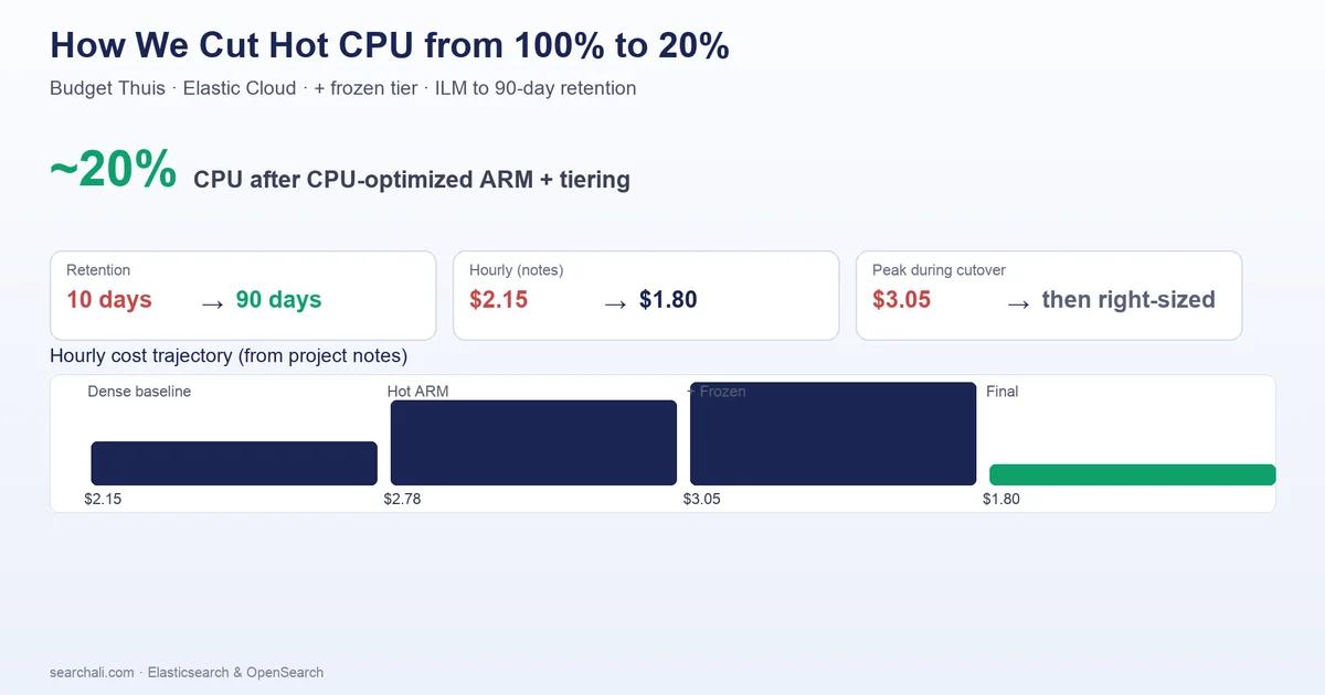
I worked with the team to stop treating symptoms and instead align hardware profile, data tiers, and index lifecycle with how observability data actually ages. The outcome was concrete: CPU pressure dropped from ~100% to ~20%, log retention increased from 10 to 90 days, and the hourly run rate moved from about $2.15/hr down to about $1.80/hr after the full sequence—including adding a frozen tier and then right-sizing the hot tier once ILM had caught up.
The Challenge
Budget Thuis runs a managed Elasticsearch stack for APM, logs, and metrics—the backbone for application and infrastructure visibility. Ingest volume was high enough that the cluster “continuously fell over” from an operations perspective: instability tied to sustained CPU saturation.
On the hot data tier, nodes were on a storage-optimized (dense) profile—great for bytes per dollar, wrong when indexing and query load dominate. The cluster was sitting at roughly 97–100% CPU while still carrying a large storage footprint. Kibana Explore and team dashboards—typically scoped to the last 7 days—felt slow because the platform was fighting for CPU headroom.
Separately, retention expectations did not match economics: the business wanted longer history than the roughly 10-day effective window for logs, without a linear explosion in hot-tier cost.
Diagnosis
Two issues stood out immediately.
Hardware–workload mismatch. Storage-dense nodes pack disks; observability workloads are often CPU-bound (indexing, merges, query fan-out, APM trace volume). When CPU pegs near 100%, you do not fix it by “waiting it out”—you change the shape of the fleet or the lifecycle of the data.
Lifecycle and tiering gap. The path to affordable long retention is not “keep everything hot forever.” It is rollover, tier movement, and delete policies that match legal and operational needs. The team needed hot data for recent troubleshooting, frozen for older-but-required history, and a disciplined delete horizon.
There were also organizational opportunities—Spaces and permissions could better isolate teams—but the burning platform issue was CPU + retention economics.
From an architecture standpoint, the cluster was multi-tenant enough for product teams to build Kibana dashboards in their own spaces—the missing piece was not “more dashboards,” it was predictable performance under ingest. Recommendations in the discovery phase also pointed at ILM hygiene: prefer rollover over rigid daily index churn where it amplifies shard overhead, and resolve stuck lifecycle transitions so data does not pile up on the wrong tier. Those themes are consistent with what we see across Elastic Cloud customers: the fleet is rarely “wrong,” but policy and hardware are often misaligned with observability traffic patterns.
The Solution
We executed a sequenced change on Elastic Cloud rather than a single big bang.
1) Move the hot tier to CPU-optimized ARM nodes. We switched the hot tier from storage-optimized dense to CPU-optimized nodes (ARM-based), trading excess disk headroom on hot nodes for vCPU capacity where the cluster was actually constrained. In this environment, that move took CPU pressure from ~100% down to ~20%—the kind of headroom that makes dashboards and ad-hoc queries predictable again.
2) Add a frozen data tier. We introduced frozen capacity so older data could live on storage-heavy, compute-light resources instead of competing with hot-tier ingestion. This is the key lever for long retention without paying hot-tier prices for cold data.
3) Update ILM to match real data aging. We aligned policy with operational reality: hot data rolls on size and time thresholds (for example, 20 GB or 2 days—exact values should match your index templates), frozen receives data older than 7 days, and delete removes beyond 90 days. That took effective log retention from 10 days to 90 days—a 9× improvement in how long teams can compare “this week vs last quarter” without exporting.
4) Right-size after ILM settled. Once data was moving across tiers as intended, we scaled down hot-node hardware to match the lower CPU pressure—bringing the hourly rate from about $3.05/hr to about $1.80/hr on the path that included frozen. Compared to the original ~$2.15/hr dense profile, the end state was still a cost reduction—not merely “more retention at any price.”
Throughout, we avoided turning case studies into credential leaks: no hostnames, queue names, or internal index naming schemes—only the architecture pattern you can replicate.
Results
| Metric | Before | After |
|---|---|---|
| Hot-tier CPU pressure | ~100% | ~20% |
| Log retention (policy outcome) | 10 days | 90 days |
| Hourly cost (reference points in project notes) | ~$2.15/hr (initial dense) | ~$1.80/hr (after final right-sizing) |
The intermediate hourly cost rose when we added more CPU and a frozen node—that is expected during a migration—then fell once ILM and tiering did their job and we could remove excess hot capacity.
If you are comparing only “before/after” hourly rates, use the same tiering context: a frozen node temporarily increases run rate while you prove lifecycle, then right-sizing captures the win. The meaningful comparison for Budget Thuis is stability + retention + cost at the end state—not the peak during cutover.
Key Takeaways
- Match hardware profile to the bottleneck. Storage-dense nodes are the wrong default when CPU and indexing dominate; CPU-optimized ARM can change the operating picture overnight.
- Long retention requires tiering. Frozen exists so you do not fund 90 days of data at hot-tier economics.
- Sequence matters. Add frozen + ILM, prove data movement, then scale down hot—otherwise you risk cutting capacity before the pipeline stabilizes.
- Observability SLAs are CPU SLAs. If Explore and dashboards are slow, check CPU saturation before tuning every query.
Need help with your Elasticsearch cluster? Reach out at searchali.com. For data tiers and long retention, see Elastic’s ILM documentation.